Recurrent Neural Networks: From Sine Waves to Shakespeare

This tutorial explores Recurrent Neural Networks (RNNs) using blox and Distrax.

We will cover two probabilistic modeling tasks:

1. Regression: Modeling a noisy sine wave using a Gaussian distribution.

2. Generation: Modeling character sequences (Shakespeare) using a Categorical distribution.

# Setup: ensure blox is importable.
import sys

sys.path.insert(0, "../src")

# Install necessary packages.
!pip install -q optax matplotlib distrax

import os

import blox as bx
import distrax
import jax
import jax.numpy as jnp
import matplotlib.pyplot as plt
import numpy as np
import optax
import requests

# Set random seed for reproducibility.
np.random.seed(0)

/usr/local/python/3.12.1/lib/python3.12/site-packages/keras/src/export/tf2onnx_lib.py:8: FutureWarning: In the future `np.object` will be defined as the corresponding NumPy scalar.
  if not hasattr(np, "object"):

Part 1: Modeling a Sine Wave (Regression)

def generate_sine_data(batch_size, seq_len):
  """Generates sine waves with random phases."""
  # Random phases for each batch element.
  phases = np.random.uniform(0, 2 * np.pi, size=(batch_size, 1))
  time = np.linspace(0, 4 * np.pi, seq_len + 1)  # +1 for target

  # Shape: (Batch, Time)
  waves = np.sin(time + phases)

  # Add channel dimension: (Batch, Time, 1)
  waves = waves[..., None]

  # Input is t, Target is t+1
  inputs = waves[:, :-1]
  targets = waves[:, 1:]
  return inputs, targets


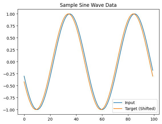
x_viz, y_viz = generate_sine_data(1, 100)
plt.plot(x_viz[0, :, 0], label='Input')
plt.plot(y_viz[0, :, 0], label='Target (Shifted)')
plt.legend()
plt.title('Sample Sine Wave Data')
plt.show()

class SineRNN(bx.Module):
  """RNN that outputs parameters for a Gaussian distribution."""

  def __init__(self, graph: bx.Graph, hidden_dim: int, rng: bx.Rng):
    super().__init__(graph)
    self.lstm = bx.LSTM(graph.child('lstm'), hidden_size=hidden_dim, rng=rng)
    # Output 2 values: mean and log_std.
    self.head = bx.Linear(graph.child('head'), output_size=2, rng=rng)

  def apply(
      self,
      params: bx.Params,
      x: jax.Array,
      prev_state: bx.LSTMState | None = None,
  ):
    # x: [Batch, Time, 1]
    (h, final_state), params = self.lstm.apply(params, x, prev_state)

    # Project to Gaussian parameters.
    out, params = self.head(params, h)
    mu, log_scale = jnp.split(out, 2, axis=-1)

    # Constrain scale to be positive.
    scale = jax.nn.softplus(log_scale) + 1e-3
    return (mu, scale), final_state, params

@jax.jit(static_argnames=['optimizer'], donate_argnames=['params', 'opt_state'])
def train_step_sine(params, opt_state, x, y, optimizer):
  trainable, non_trainable = params.split()

  def loss_fn(trainable):
    curr_params = trainable.merge(non_trainable)
    (mu, scale), _, new_params = sine_model.apply(curr_params, x)

    # Maximize Log Likelihood of the Gaussian.
    dist = distrax.Normal(loc=mu, scale=scale)
    loss = -dist.log_prob(y).mean()

    _, new_non_trainable = new_params.split()
    return loss, (loss, new_non_trainable)

  grads, (loss, new_non_trainable) = jax.grad(loss_fn, has_aux=True)(trainable)
  updates, new_opt_state = optimizer.update(grads, opt_state, trainable)
  new_trainable = optax.apply_updates(trainable, updates)
  return new_trainable.merge(new_non_trainable), new_opt_state, loss


# Create model components.
graph = bx.Graph('net')
rng = bx.Rng(graph.child('rng'))
sine_model = SineRNN(graph.child('sine_rnn'), hidden_dim=32, rng=rng)

# Initialize with sample data shape.
sample_x, _ = generate_sine_data(batch_size=1, seq_len=50)
sine_params = rng.seed(bx.Params(), seed=42)
_, _, sine_params = sine_model.apply(sine_params, sample_x)
sine_params = sine_params.locked()

# Train.
optimizer = optax.adam(1e-2)
opt_state = optimizer.init(sine_params.split()[0])

losses = []
for i in range(1000):
  x, y = generate_sine_data(batch_size=32, seq_len=50)
  sine_params, opt_state, loss = train_step_sine(
      sine_params, opt_state, x, y, optimizer
  )
  losses.append(loss)
  if i % 100 == 0:
    print(f'Step {i}, NLL: {loss:.4f}')

plt.plot(losses)
plt.title('Sine Wave Training NLL')
plt.show()

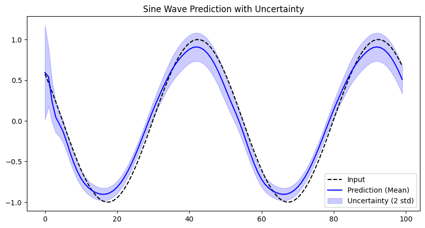
# Visualize predictions.
x_test, y_test = generate_sine_data(1, 100)
(mu, scale), _, _ = sine_model.apply(sine_params, x_test)

t = np.arange(100)
plt.figure(figsize=(10, 5))
plt.plot(t, x_test[0, :, 0], 'k--', label='Input')
plt.plot(t, mu[0, :, 0], 'b-', label='Prediction (Mean)')
plt.fill_between(
    t,
    mu[0, :, 0] - 2 * scale[0, :, 0],
    mu[0, :, 0] + 2 * scale[0, :, 0],
    color='b',
    alpha=0.2,
    label='Uncertainty (2 std)',
)
plt.legend()
plt.title('Sine Wave Prediction with Uncertainty')
plt.show()

Part 2: Tiny Shakespeare (Generation)

Now we apply the same principles to character generation using a Categorical distribution.

def download_data():
  url = 'https://raw.githubusercontent.com/karpathy/char-rnn/master/data/tinyshakespeare/input.txt'
  if not os.path.exists('input.txt'):
    data = requests.get(url).text
    with open('input.txt', 'w') as f:
      f.write(data)
  else:
    with open('input.txt', 'r') as f:
      data = f.read()
  return data


text = download_data()
chars = sorted(list(set(text)))
vocab_size = len(chars)
stoi = {ch: i for i, ch in enumerate(chars)}
itos = {i: ch for i, ch in enumerate(chars)}


def encode(s):
  return [stoi[c] for c in s]


def decode(indices):
  return ''.join([itos[i] for i in indices])


data = jnp.array(encode(text), dtype=jnp.uint32)
train_data = data[: int(0.9 * len(data))]


def get_batch(batch_size=64, block_size=128):
  ix = np.random.randint(0, len(train_data) - block_size, size=(batch_size,))
  x = jnp.stack([train_data[i : i + block_size] for i in ix])
  y = jnp.stack([train_data[i + 1 : i + block_size + 1] for i in ix])
  return x, y

class CharRNN(bx.SequenceBase):

  def __init__(
      self,
      graph: bx.Graph,
      vocab_size: int,
      embed_dim: int,
      hidden_dim: int,
      rng: bx.Rng,
  ):
    super().__init__(graph)
    self.rng = rng
    self.embed = bx.Embed(
        graph.child('embed'),
        num_embeddings=vocab_size,
        embedding_size=embed_dim,
        rng=rng,
    )
    self.lstm = bx.LSTM(graph.child('lstm'), hidden_size=hidden_dim, rng=rng)
    self.head = bx.Linear(graph.child('head'), output_size=vocab_size, rng=rng)

  def __call__(
      self, params: bx.Params, inputs: jax.Array, prev_state: bx.LSTMState
  ):
    # Single step for generation.
    x_emb, params = self.embed(params, inputs)
    (x_hidden, new_state), params = self.lstm(params, x_emb, prev_state)
    logits, params = self.head(params, x_hidden)
    return (logits, new_state), params

  def apply(
      self,
      params: bx.Params,
      x: jax.Array,
      prev_state: bx.LSTMState | None = None,
  ):
    # Sequence processing for training.
    x_emb, params = self.embed(params, x)
    (x_seq, final_state), params = self.lstm.apply(params, x_emb, prev_state)
    logits, params = self.head(params, x_seq)
    return (logits, final_state), params

  def initial_state(self, params: bx.Params, inputs: jax.Array):
    return self.lstm.initial_state(params, inputs)

@jax.jit(static_argnames=['optimizer'], donate_argnames=['params', 'opt_state'])
def train_step_char(params, opt_state, x, y, optimizer):
  trainable, non_trainable = params.split()

  def loss_fn(trainable):
    curr_params = trainable.merge(non_trainable)
    (logits, _), new_params = char_model.apply(curr_params, x)

    # Categorical Log Likelihood.
    dist = distrax.Categorical(logits=logits)
    loss = -dist.log_prob(y).mean()

    _, new_non_trainable = new_params.split()
    return loss, (loss, new_non_trainable)

  grads, (loss, new_non_trainable) = jax.grad(loss_fn, has_aux=True)(trainable)
  updates, new_opt_state = optimizer.update(grads, opt_state, trainable)
  new_trainable = optax.apply_updates(trainable, updates)
  return new_trainable.merge(new_non_trainable), new_opt_state, loss


# Create model components.
graph = bx.Graph('net')
char_rng = bx.Rng(graph.child('rng'))
char_model = CharRNN(
    graph.child('char_rnn'),
    vocab_size=vocab_size,
    embed_dim=64,
    hidden_dim=256,
    rng=char_rng,
)

# Initialize with sample data shape.
sample_x, _ = get_batch(batch_size=1, block_size=128)
char_params = char_rng.seed(bx.Params(), seed=42)
_, char_params = char_model.apply(char_params, sample_x)
char_params = char_params.locked()

# Train.
optimizer = optax.adamw(3e-4)
trainable, _ = char_params.split()
opt_state = optimizer.init(trainable)

losses = []
print('Training CharRNN...')
for step in range(1000):
  x, y = get_batch()
  char_params, opt_state, loss = train_step_char(
      char_params, opt_state, x, y, optimizer
  )
  losses.append(loss)
  if step % 100 == 0:
    print(f'Step {step}, NLL: {loss:.4f}')

plt.plot(losses)
plt.title('CharRNN NLL')
plt.show()

def generate(params, start_str, length=200, temperature=1.0):
  context = jnp.array([encode(start_str)], dtype=jnp.int32)
  state, params = char_model.initial_state(params, context)

  # Warmup.
  (logits_seq, state), params = char_model.apply(params, context, state)
  next_logits = logits_seq[:, -1]

  generated = []
  for _ in range(length):
    key, params = char_rng(params)
    dist = distrax.Categorical(logits=next_logits / temperature)
    next_token = dist.sample(seed=key)
    generated.append(int(next_token[0]))

    (next_logits, state), params = char_model(params, next_token, state)

  return start_str + decode(generated)


print('Generated Text (temperature=1.0):')
print(generate(char_params, 'ROMEO: '))
print('Generated Text (temperature=0.1):')
print(generate(char_params, 'ROMEO: ', temperature=0.1))

Generated Text (temperature=1.0):
ROMEO: By?,
I decs is thiigd.

SIMENRLETI:
Tey nore gree.

WPORENY:
Morves nov meant aidt asaner?

Lith Meray:
Qurd now!
The pobnet brosed; I mifmeany seel andtrat! and were gombe aftire;
Vorgich stoue yous
Generated Text (temperature=0.1):
ROMEO: I will the mand the mand the sores the mand the mand and and the the the the the the and the the the the sorest the mand the bronger the will the sorest the hare the the beather the the hare the hare